In the example I give correct bootstrap and Bayesian bootstrap procedures and wrong ones. The wrong Bayesian bootstrap follows description from Chernick (2008), page 122 (that is equivalent to the comment to my last post).
Here is the code that I used:
library(gtools)
ok.mean.bb <- function(x, n) {
apply(rdirichlet(n, rep(1,length(x))), 1, weighted.mean,
x = x)
}
ok.mean.fb <- function(x, n) {
replicate(n, mean(sample(x, length(x), TRUE)))
}
wrong.mean.bb <- function(x, n) {
replicate(n, mean(sample(x, length(x), TRUE,
diff(c(0, sort(runif(length(x) - 1)), 1)))))
}
wrong.mean.fb <- function(x, n) {
replicate(n, mean(sample(sample(x, length(x), TRUE),
length(x), TRUE)))
}
set.seed(1)
reps <- 10000
x <- cars$dist
par(mar=c(5,4,1,2))
plot(density(ok.mean.fb(x, reps)), main = "", xlab = "Bootstrap
mean")
lines(density(ok.mean.bb(x, reps)), col = "red")
lines(density(wrong.mean.fb(x, reps)), col = "blue")
lines(density(wrong.mean.bb(x, reps)), col = "green")The figure it produces is:
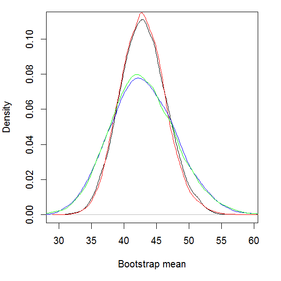
Black curve is standard bootstrap density, red is Bayesian bootstrap and blue and green are generated by wrong bootstrapping procedures (respectively frequentist and Bayesian).
We can see that wrong Bayesian bootstrap has an equivalent in standard bootstrap approach that is generated by repeating the sampling twice (sampling from a sample) and it clearly increases dispersion of the results.
FYI, there is an implementation of Rubin's Bayesian bootstrap called "BayesianBootstrap" in the LaplacesDemon package of R, available on CRAN. I do not know which side they come down on the question of how the first bootstrap should be sampled, as I have not dug into the problem. Perhaps the LaplacesDemon implementation will add a third voice to the discussion.
ReplyDeleteI don't think Rubin's "Bayesian bootstrap" is used as much because it seems to simple confuse matters with stylistic distractions. Apparently, it has use in cases of censoring, e.g., for imputation. Efron discusses it in passing in his "Second thoughts on the Bootstrap" from 2003.
BayesianBootstap in LaplacesDemon simply replicates standard bootstrap procedure in disguise not Bayesian bootstrap.
ReplyDeleteYou can see it in the following part of the source code:
for (s in 1:S) {
if (s%%Status == 0)
cat("\nBootstrapped Samples:", s)
u <- c(0, sort(runif(N - 1)), 1)
g <- diff(u)
X.B[s, ] <- X[sample(1:N, 1, prob = g, replace = TRUE),
]
}
In each step of the loop only one observation is sampled (size parameter is equal to 1). And we notice that u and g are resampled every time in the loop also.
Therefore in each step of the loop is observation is sampled with probability 1/N. This is a standard bootstrap procedure.
To see this notice for example that running:
BayesianBootstrap(1:10,1)
10 times is equivalent to running:
BayesianBootstrap(1:10,10)
Hi Bogumil,
ReplyDeleteThanks for showing this to me.
I think the two approaches here, rdirichlet and differenced sampling weights, are equivalent. The difference in the results, such as between ok.mean.bb and wrong.mean.bb, is due to repeated sampling in wrong.mean.bb with the same sampling weights. According to Chernik (2008), page 122:
"A second Bayesian bootstrap replication is generated in the same way, but
with a new set of n - 1 uniform random numbers and hence a new set of g[i]'s."
In wrong.mean.bb, the size argument of length(x) returns multiple draws, but each of these draws has the same sampling probabilities. I believe Chernik is using the word replication to refer to each draw, which could be confusing to readers here who observe the replicate function is used here for each collection of length(x) draws. My interpretation of Rubin (1981) and Chernik (2008) is that the sampling probabilities should be refreshed for each draw.
The BayesianBootstrap function in the LaplacesDemon package seems to be working correctly (whew!). For example, I see the same approximate results by substituting:
ok.mean.bb <- function(x, n) {
replicate(n, mean(BayesianBootstrap(x, length(x))), TRUE)
}
As a side note, the rdirichlet function in LaplacesDemon is much faster than that currently implemented in gtools. The BayesianBootstrap function is not using rdirichlet at the moment, and calculates it exactly as presented by Rubin (1981). The rdirichlet approach presented here is much faster.
One thing I discovered by working through this is that the current BayesianBootstrap function returns "The Bayesian Bootstrap has finished." numerous times
Before you run this example (and fill your screen with these messages!), I suggest replacing this line of source code in BayesianBootstrap:
cat("\n\nThe Bayesian Bootstrap has finished.\n\n")
with
if(Status < S) cat("\n\nThe Bayesian Bootstrap has finished.\n\n")
I will update this in the package for the next version.
Thanks again for pointing this discussion out to me.
In my opinion BayesianBootstrap it is not working correctly - it simply reproduces standard bootstap.
DeleteTo see this consider the following example:
library(gtools)
library(LaplacesDemon)
ok.mean.bb <- function(x, n) {
apply(rdirichlet(n, rep(1,length(x))), 1, weighted.mean, x = x)
}
ok.mean.fb <- function(x, n) {
replicate(n, mean(sample(x, length(x), TRUE)))
}
demon.mean.bb <- function(x, n) {
replicate(n, mean(BayesianBootstrap(x, length(x))), TRUE)
}
set.seed(1)
reps <- 10000
x <- 1:2
par(mar=c(5,4,1,2))
plot(density(ok.mean.fb(x, reps)), main = "", xlab = "Bootstrap mean", lwd=3)
lines(density(ok.mean.bb(x, reps)), col = "red")
lines(density(demon.mean.bb(x, reps)), col = "green")
As you can see green line (BayesianBootstrap) is exactly the same as black (standard bootstrap). However, Bayesian bootstrap (red) is smooth - and should be smooth, because this is exactly the difference between sampling from Dirichlet and multinomial distribution.
Now going back to Rudin (1981) look at the following passage:
"For example with \phi=mean of X, in each BB replication we calculate the mean of X as if g_i were the probability that X=x_i; that is we calculate sum_{1}^{n}g_ix_i. The distribution of the values of \sum_{1}^{n} over all BB replications (i.e. generated by repeated draws of the g_i) is the BB distribution of the mean of X."
So you should sample g_i and calculate weighted mean using them.
If the BayesianBootstrap function is not working correctly in LaplacesDemon, I will gladly correct it, and have recently opened a forum for the public discussion of development, including bugs.
ReplyDeleteIn this case, however, I think it is correct.
On the following page, Rubin shows in figure 1 a comparison between the BB and the bootstrap for correlation, and the results are very similar.
When I run the code in the previous comment, the BayesianBootstrap function estimates a distribution of the mean that is remarkably similar to the frequentist bootstrap. The ok.mean.bb function returns a distribution with stunning uncertainty, especially given 10,000 replications.
I see an article called "A large Sample Study of the Bayesian Bootstrap" (1987) by Albert Lo. Throughout the article, Lo notes the large sample properties are very similar between the bootstrap and the BB, and Lo is referring to large samples of replicates.
I think the BayesianBootstrap function is doing what Lo shows on the first page of his article, in steps 2 and 3, and that a test statistic such as the mean is calculated as such on the bootstrapped samples. Please let me know if this is incorrect. Thanks.
I know Lo (1987) article and this is how I understand it:
Deletea) n denotes original (data) sample size
b) B denotes number of bootstrap replicates
c) when Lo talks about convergence (for instance top of page 362) it is indicated that the convergence rate is n^{1/2} which clearly relates to data sample size (not bootstrap size)
d) Finally going back to steps 1, 2 and 3 on page 360. In step 1 a DISTRIBUTION is generated (denoted D_n). In step 2 large numer of DISTRIBUTIONS is generated using step 1 (D_{n1},...,D_{nB}). For each distribution FUNCTIONAL \theta is evaluated. In my opinion this does not involve sampling. For example in equation (1.4) only one sampling is performed (to obtain D_n in step 1). Similarly in equation (4.1) for mean we can see that functional g_1 depends only on D_n.
In summary in my opinion: (1) the procedure from steps 1 to 3 involves sampling only in step 1 and (2) large sample means large n (number of original obserwations).
The code in the previous comment shows differences because I wanted to set number of observations (n) small, because then there the difference between Bayesian and standard boostrap is noticeable. Replacing
x <- 1:2
by
x <- 1:10
in the example already makes all the distributions very similar (because sample size is increased).
And you can check that the code of BayesianBootstap in LaplacesDemon does not APPROXIMATE standard bootstrap but is EXACTLY the same procedure by running it for large number of replications of bootstrap (B) for different initial data sets.
Additionally you can look at original Rubin (1981) example data. Here is the code:
ReplyDeletelibrary(LaplacesDemon)
dye <- c(1.15, 1.7, 1.42, 1.38, 2.8, 4.7, 4.8, 1.41, 3.9)
efp <- c(1.38, 1.72, 1.59, 1.47, 1.66, 3.45, 3.87, 1.31, 3.75)
data.set <- data.frame(dye,efp)
sboot <- function() {
cor(data.set[sample(1:9, replace=T),])[1,2]
}
bboot <- function() {
cov.wt(data.set, diff(c(0,sort(runif(8)),1)), cor=T)$cor[1,2]
}
dboot <- function() {
cor(BayesianBootstrap(data.set, 9))[1,2]
}
set.seed(1)
par(mfrow=c(1,3))
hist(replicate(10000, sboot()), breaks=seq(-1,1, len=101), xlim=c(0.4,1))
hist(replicate(10000, bboot()), breaks=seq(-1,1, len=101), xlim=c(0.4,1))
hist(replicate(10000, dboot()), breaks=seq(-1,1, len=101), xlim=c(0.4,1))
You can see that dboot() looks like sboot() but not like bboot(). And in Rubin (1981) we can see that Bayesian bootstap should have less extreme results (near 1 and below 0.8). This can be seen in bboot() only.
Good stuff.
ReplyDeleteWe may need a tie-breaker on the Lo article, because the way I read it:
Step 1 involves drawing the sampling probabilities from gaps from uniforms, and then
Step 2 involves drawing the bootstrap sample, though step 1, the sampling probabilities, are drawn for each bootstrap sample in step 2.
This agrees again with Chernik (2008), page 122:
"A second Bayesian bootstrap replication is generated in the same way, but wit ha new set of n - 1 uniform random numbers and hence a new set of g[i]'s."
The bboot in the above example does not do that. But I do like the look of your static-g bboot better for that last example though!
It's ok if we disagree over whether the main thrust of the Lo aricle is on data or bootstrap asymptotics (I'd suggest the last sentence of the first page, p. 360, supports bootstrap though), but the first thing to nail down is that the gaps are drawn for each bootstrap replicate.
I am wondering why you'd say that the BayesianBootstrap function doesn't approximate, but is exactly the same, when the probabilities g are not 1/n like in the bootstrap. I'm scratching my head on that one.
There may be other interesting things to explore here, but let's start with whether or not the gaps, calculated from uniform sampling, should differ for each bootstrap replication.
In my opinion gaps calculated from uniform sampling should differ for each bootstrap replication
DeleteBUT should be the same in one bootstrap replicate (i.e. generation of D_n in Lo, 1986).
The key here is that one boostrap replicate allows us to calculate the value of functional \theta(D_n,X). So it is equivalent to sampling N observations with replacement in standard bootstrap.
The last sentence on page 360 means in my opinion refers to large B but it says that step 3 approximates POSTERIOR DISTRIBUTION well for large B. And the issue is what happens for large n, citing last paragraph on page 362: "(...) a unified treatment of the asymptotic theory can be achieved by studing the behavior of d_n=n^{1/2}{D_n-F_n} for large n's.".
Finally going back to the BayesianBootstrap function. The piece of code:
u <- c(0, sort(runif(N - 1)), 1)
g <- diff(u)
X.B[s, ] <- X[sample(1:N, 1, prob = g, replace = TRUE), ]
is crucial. It is repeated S times INDEPENDENTLY. Notice that in single step of the loop each row of the data has the probability of chosing equal to 1/N. And because each step of the loop is independent from others we can see that the procedure performs unweighted sampling with replacement (so it is standard bootstrap).
After carefully re-reading these articles from your perspective, I'm convinced you're right. I will correct the BayesianBootstrap function, and will also extend it to produce statistics rather than strictly samples. If it sounds good, I will email it to your for your feedback. Many thanks again for pointing this out to me.
ReplyDelete